Cognitave Inc.
MXD
Design, Data, Work-flows
Dynamic Mathematics Link>>
Quantum Logic Trainings>>
MAQM>>
CAED>>.

-
Carey Mead
Misha Mohawold
Caltech Tech Ui
-
Automotive Level 2-4
-
Catastrophe Theory
-
Applied Quantum Mechanics
-
Information Design and Visualization
Design of Everyday Things
Design for Human affairs
Power Shift
Reserved Copyright 2023 All Rights reserved for contained herein by United States of America Laws and Regulations and Internationally. All relevant Copyrights, all proprietary and specially trademarks are reserved and enforced through proper legal routes. Maxdi Inc. Cognitave Inc. Copyright 2023.
Maxdi.com https://cognitave.com
⊗∴⊛⊛⊡⊡ ⨥⨠⨻⩒⩒


⊗∴⊛⊛⊡⊡ ⨥⨠⨻⩒⩒

\chapter{References}
\begin{thebibliography}{1}
	\bibitem {1}
	Ridenour, Louis Nicot, ed. Radar system engineering. Vol.~1. Dover Publications, 1965.
	\bibitem {2}
	Kissinger, Dietmar. Millimeter-wave receiver concepts for 77 GHz automotive radar in silicon-germanium technology. Springer Science \& Business Media, 2012.
	\bibitem {3}
	Karnfelt, C. et al., “77 GHz ACC Radar Simulation Platform”, IEEE International Conferences on Intelligent Transport Systems Telecommunications (ITST), 2009.
	\bibitem {4}
	Rohling, H. and M. Meinecke., “Waveform Design Principle for Automotive Radar Systems”, Proceedings of CIE International Conference on Radar, 2001.
	\bibitem {5}
	A. Stove, “Linear FMCW radar techniques”, IEE Proceedings of Radar and Signal Processing, vol. 139, no. 5, pp. 343–350, 1992.
	\bibitem {6}
	I. V. Komarov and S. M. Smolskiy, Fundamentals of Short-Range FM Radar. Boston, MA: Artech House, 2003.
	\bibitem {7}
	Gardill, Markus. "Characterization and Design of Small Array Antennas for Direction-Of-Arrival Estimation for Ultra-Wideband Industrial FMCW Radar Systems." (2015).
	\bibitem {8}
	Merrill Skolnik, Introduction to Radar Systems, 3rd Edition, McGraw-Hill, 2001
	\bibitem {9} \tt {http://www.yole.fr/} %Radar\_AutomotiveLandscape.aspx#.W1DrJS3Gzow
	\bibitem {10} \tt {http://www.microwavejournal.com/}
	\bibitem {11} \tt {https://www.microwaves101.com/}
	\bibitem {20} \tt {https://www.ims2016.org}
	% \\ Dissertation Link
	\bibitem {30} \tt{ https://www.linkedin.com/in/maxdi}
	% COMPANY WEBISTES
	\bibitem {40} \tt {http://www.maxdi.com/} % MXD
	\bibitem {50} \tt {http://www.cognitave.com/} %COGN
	% COMPANY WEBISTES
	\bibitem {412} \tt {https://www.instagram.com >> @maxdinyc} % MXD
	\bibitem {40} \tt {https://www.instagram.com >> @maxdiinc} %COGN
	\bibitem {40} \tt {https://www.instagram.com >> @maxdisystems} %COGN
	\bibitem {40} \tt {https://www.tiktok.com/en >> @mxdnyc} % UGI - MXD STR		 %articles/29958-mwj-talks-adi-and-autoliv-about-advanced-automotive-radar-sensors-and-rides-in-test-car
\end{thebibliography}
QLAP
-
Input Database links..
Octave* download page
Octave* Documentations
Octave* Demos
-
RF\&MW Simulation and Modelling
EM Radiation Phenomenal Analysis
ANSYS HFSS CIRCUITS
EMPRO $KEYSADS AWR KiCAD
-
RADAR Sensing
Automotive Tiers Vendors
#Lidar #Radar #Cameras #Ultrasound #ActiveSafety #SAvinglives

⊗∴⊛⊛⊡⊡ ⨥⨠⨻⩒⩒
%% Inout Data for DoA Estimation with ANN
% Cognitave, Inc.
% Programmer: Mahdi Haghzadeh, CEO
% Revisions:
% Date: 1/15/2018
%% Modeling the Received Array Signals
% Define a uniform linear array (ULA) composed of 10 isotropic antennas. The
% array element spacing is 0.5 meters.
N = 10;
ula = phased.ULA('NumElements',N,'ElementSpacing',0.5);
%%
% Simulate the array output for one incident signal. The signal is incident
% from 90∞ in azimuth. It's elevation angles is randomly generated. We assume
% that the directione are unknown and need to be estimated. Simulate the
% baseband received signal at the array demodulated from an operating frequency of 300 MHz.
fc = 76.5e9; % Operating frequency
fs = 8192; % Sampling frequency
lambda = physconst('LightSpeed')/fc; % Wavelength
pos = getElementPosition(ula)/lambda; % Element position in wavelengths
%rs = rng(2012); % Set random number generator
randAng = randi(90)
ang1 = [randAng, 0]; % Direction of the signals
angs = ang1;
Nsamp = 1024; % Number of snapshots
noisePwr = 0.01; % Noise power
signal = sensorsig(pos,Nsamp,angs,noisePwr);
%%
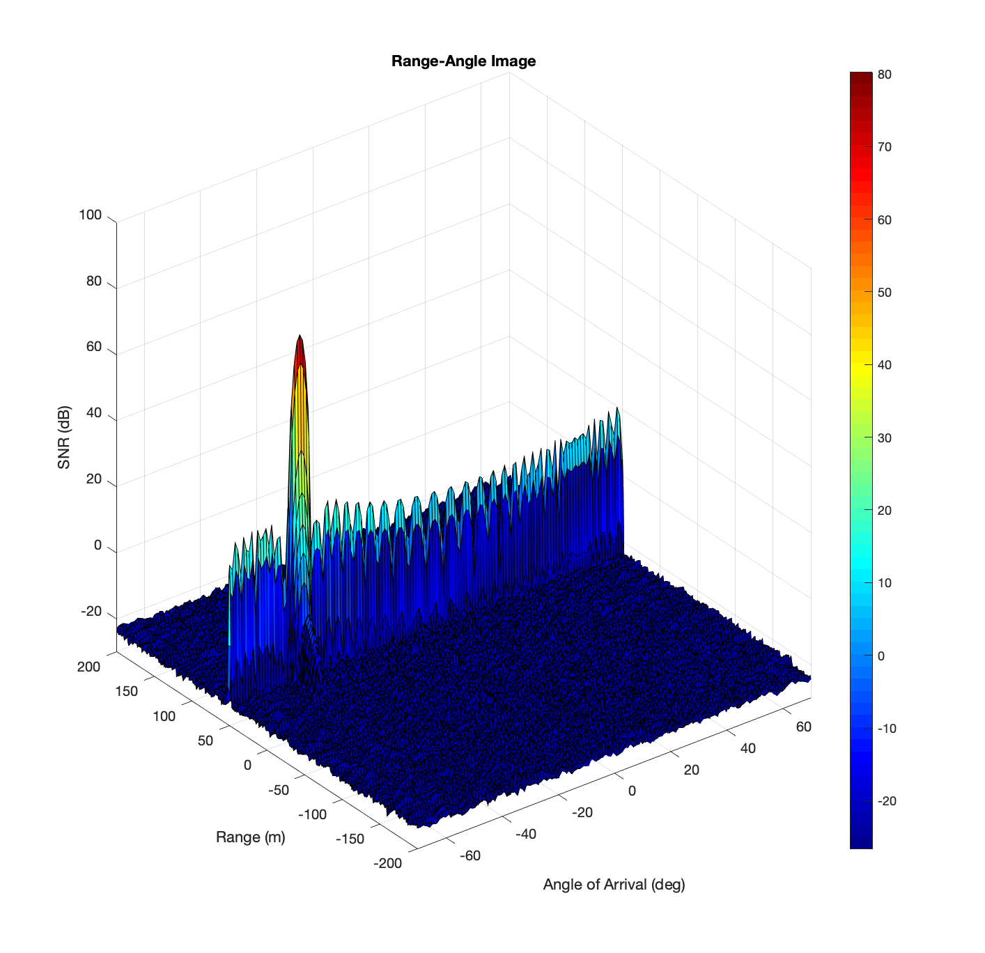
% Because a ULA is symmetric around its axis, a DOA algorithm cannot uniquely
% determine azimuth and elevation. Therefore, the results returned by these high-resolution
% DOA estimators are in the form of broadside angles. An illustration of broadside
% angles can be found in the following figure.
%
%
%
% Calculate the broadside angles corresponding to the two incident angles.
ATT: Maxdi Inc.> 90 West St, Suite 16K
New York, NY 10006


Markets & Partner Clients
-
RF/MW Engineering, Electronics, Neuro-analog (Neuromorphic) Computing, Automotive Radar, Radar sensing and monitoring, quantum computing, mathematical modeling
-
Design flow software and techniques, Simulation baed modeling and analysis, optimizations and predictions, validation and verification work-flows
-
Aerospace & Defense, Automotive Sensing (Radar, Lidar, Vision, Ultrasonic), Software Design, Finance, Legal
-
Matlab (Mathworks Inc), Mathematica (Wolfram), Octave8, SPICE (LT-Spice, Q-Spice), HFSS (Ansoft), ADS (Keysight), Simulink (Mathworks), AWR (Cadence), Pyton


VE
Cognitave inc, ($COGN)
MXD ($Mxd) the informational tag code for Maxdi Inc.
COGN ($Cogn) the informational tag code for Maxdi Inc.
Across platforms Maxdi.com and cognitive.com \\
Copyright 2024. All rights reserved.